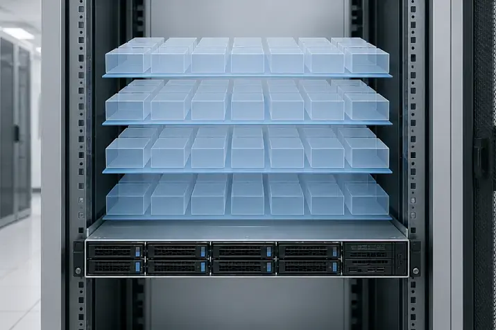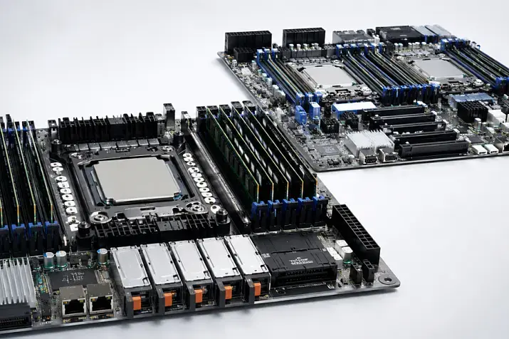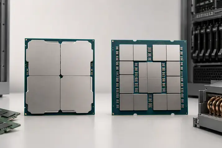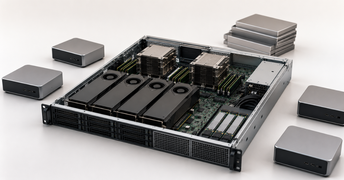
An LLM inference server is sized using more than the model size alone. First, determine the actual length of input prompts and responses, the peak request rate, the number of requests processed simultaneously, and the acceptable latency. Then calculate memory for the model weights and KV cache separately, estimate token throughput, and only after that select the GPU, CPU, RAM, NVMe storage, and network. A small internal chatbot may need only one accelerator, while the same model with a long context and dozens of active conversations may require several GPUs or multiple server replicas.
Model + context + active requests + target latency + reserve = server configuration.
The model itself may fit completely into GPU memory, yet the service can still start rejecting requests as the load grows. This happens because memory is used not only for weights. A significant share is occupied by the KV cache, temporary buffers, service structures, and data used by the software environment.
The number of users by itself also says very little. One hundred employees who use a chatbot several times a day create a very different load from twenty customers who simultaneously submit large documents and expect detailed answers.
GPU servers
Free shipping on orders over £500 in the EU, £500 in the UK, and $3,000 in the USA
Free shipping on orders over £500 in the EU, £500 in the UK, and $3,000 in the USA

Free shipping on orders over £500 in the EU, £500 in the UK, and $3,000 in the USA
Free shipping on orders over £500 in the EU, £500 in the UK, and $3,000 in the USA
Why model size is not enough
When selecting a server, you need to check four independent constraints.
Capacity
GPU memory must simultaneously hold the weights, the KV cache for active requests, temporary buffers, service structures, and a reserve for fragmentation. Starting the model without users only confirms that the minimum data set fits.
Latency and throughput
The user first waits for the context to be processed and for the first part of the response, and then for the rest of the generation. A test with a 500-token context cannot be extrapolated to a workload with 8,000 or 16,000 tokens.
The server must also process the incoming flow faster than the queue grows. Performance therefore needs to be measured at specified input and output lengths, concurrency levels, and latency limits.
Scaling
There are three possible architectures:
- One model is split across several GPUs.
- Several independent copies of the model are running.
- The model or its replicas are distributed across servers.
Model parallelism is required when the model does not fit on a single accelerator. Replicas are better for increasing the number of users served and improving fault tolerance. A multi-node design is used when one server does not provide enough resources, but it requires a fast network and more complex management.
What data is needed for the calculation
For an existing application, take the parameters from request logs. For a new project, prepare three profiles: normal, peak, and adverse but still acceptable.
| Parameter | What to measure | What it affects |
|---|---|---|
| Model | Parameters, layers, KV heads, head size | Model weight size and KV cache |
| Weight format | 16, 8, or 4 bits | GPU memory usage |
| Context | Median, 95th percentile, and limit | Time to first token and KV cache |
| Response | Average length, 95th percentile, and limit | Request duration and output throughput |
| Rate | Requests per second or minute at peak | Concurrency and queue size |
| Latency | First token, token intervals, total time | GPU class and number of replicas |
| Availability | Acceptable downtime | Redundancy |
| Growth | Load in 6–12 months | Platform headroom |
Context should be measured with the tokenizer of the specific model. Converting characters or words into tokens is inaccurate because tokenisation depends on the language and vocabulary.
The model's advertised maximum context should not be assigned to every request. The calculation needs the actual length distribution and a product-level limit. An average is also insufficient: if five per cent of requests are substantially longer than the rest, a configuration based on the average will degrade latency precisely for the heaviest part of the workload.
How to calculate memory for model weights
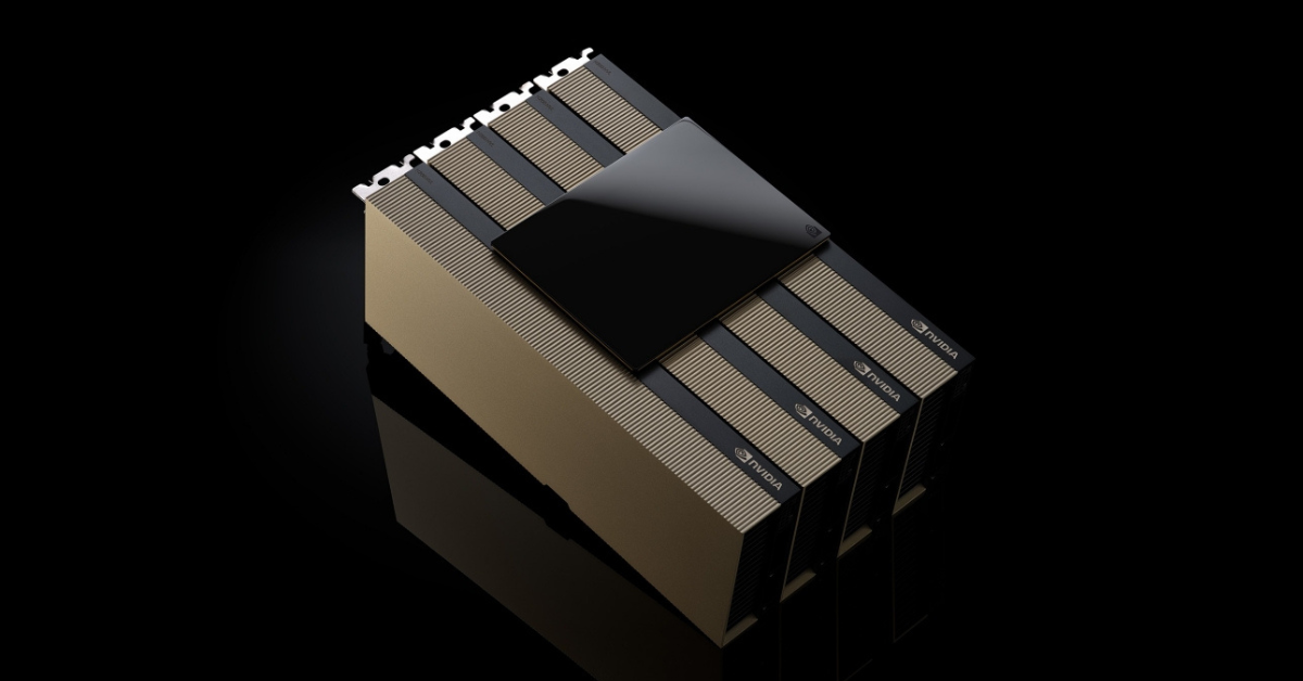
NVIDIA H200 is an example of a server GPU with a large amount of high-speed memory. Source: NVIDIA.
Image source: NVIDIA
The preliminary weight size is calculated using the following formula:
Weight memory ≈ number of parameters × bits per parameter ÷ 8
For a quick estimate:
- 7 billion parameters in a 16-bit format — about 14 GB;
- 14 billion — about 28 GB;
- 32 billion — about 64 GB;
- 70 billion — about 140 GB;
- 70 billion in an 8-bit format — about 70 GB;
- 70 billion in a 4-bit format — about 35 GB.
This is the theoretical size of the weights alone. Hugging Face recommendations for inference optimisation cover quantisation and other ways to reduce memory consumption, but the total service footprint cannot be determined by a single formula.
Add the following to the weights:
- quantisation scales and metadata;
- temporary tensors and library workspaces;
- memory for execution graphs;
- the KV cache;
- scheduler structures;
- fragmentation;
- headroom for stable operation during peak loads.
For this reason, you should not choose an accelerator on the assumption that the weights can occupy almost all available memory. Even if the model starts, there may be no room left for context and concurrent requests.
What quantisation changes
Converting weights from 16 bits to 4 bits theoretically reduces their size by about four times, but total memory usage does not fall by the same factor. The KV cache may still be stored in a 16- or 8-bit format, while buffers and some operations may use higher precision.
There are other limitations:
- different models lose quality to different degrees;
- the format must be supported by the selected environment and GPU;
- a 4-bit model is not necessarily faster than an 8-bit model;
- format conversion can sometimes reduce the performance gain;
- mixture-of-experts models usually keep all expert weights in memory, although only some of them are active for a single token.
Quantisation primarily solves a capacity problem. Its effect on quality and speed must be tested on production requests.
Choosing the Right Equipment
Our specialists will contact you and answer all your questions
KV cache: how context and concurrent requests consume memory
During generation, the model stores intermediate keys and values for tokens that have already been processed. This means the entire preceding context does not need to be recalculated for every new token. This data is called the key-value cache, or KV cache.
The cache grows with the sequence and exists separately for every active request. It includes both the input-context tokens and the portion of the response already generated.
For common transformer architectures, the following approximate formula is used:
KV cache = 2 × number of layers × number of KV heads × head size × bytes per element × tokens × active sequences
The factor of 2 accounts for keys and values. The number of KV heads must be taken from the model configuration rather than replaced with the total number of attention heads. Paged allocation, block reuse, and cache limits are described in the TensorRT-LLM documentation.
Example for a hypothetical 70-billion-parameter model
Assume the following architecture:
- 80 layers;
- 8 KV heads;
- head size of 128;
- 2 bytes per element.
One token in one sequence requires:
2 × 80 × 8 × 128 × 2 = 327,680 bytes, or approximately 0.3125 MiB.
This gives:
- 8,192 tokens use about 2.5 GiB for one sequence;
- 16,384 tokens use about 5 GiB;
- 16 sequences of 8,192 tokens use about 40 GiB;
- 32 sequences of 16,384 tokens use about 160 GiB.
The weights of a 4-bit model theoretically use about 35 GB. However, with sixteen long concurrent requests, the combined weight and KV-cache footprint already approaches 75 GB before buffers and reserve are included. On an accelerator with 80 GB of memory, this configuration will be close to the capacity limit even though the idle model occupies less than half of the memory.
KV-cache consumption is usually reduced in several ways:
- limit the working context;
- summarise or remove old conversation history;
- set a maximum response length;
- reduce the number of active sequences per replica;
- use a more compact cache format when supported;
- use paged memory allocation;
- reuse identical request prefixes;
- separate long-running background tasks from the interactive queue.
For RAG, it is especially important to control the number and size of retrieved chunks. Passing all search results into the prompt increases both the KV cache and input-processing time. Additional reranking is often more efficient than simply increasing the context.
How to convert user numbers into active requests
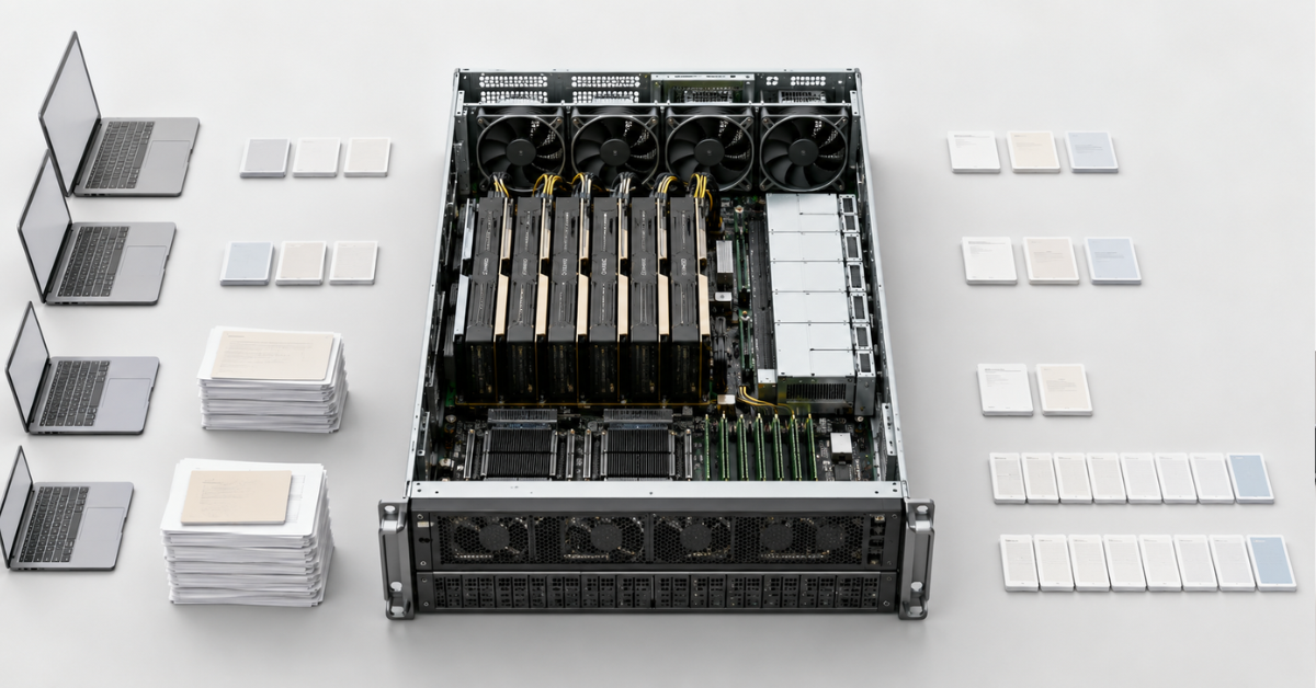
For the server, registered users are less important than requests waiting in the queue, undergoing context processing, or currently being generated.
Active requests ≈ peak arrival rate × average processing time
If one request arrives per second and the response takes 20 seconds to generate, approximately 20 requests are being served simultaneously. If the processing time increases to 40 seconds, the concurrent load doubles at the same arrival rate.
Account for short peaks, the full duration of streamed responses, long requests, client limits, and prompt cancellation when generation is no longer needed. Retries after timeouts are also dangerous: during overload, they create additional requests.
One thousand employees may produce only two or three active conversations, while a handful of large API customers may continuously keep dozens of sequences active.
Which latency metrics to measure
There is no single universal latency metric for an LLM service. Three measurements matter for an interactive application.
Time to first token
This is the period from submitting a request to receiving the first part of the response. It includes queueing, tokenisation, input-context processing, and the start of generation. This metric is particularly noticeable in a chatbot: progressively displayed text feels normal, while a long period with no output feels like the application has frozen.
Inter-token latency
This indicates how smoothly the rest of the response is generated. It is affected by model size, GPU memory bandwidth, batching, competition between requests, and communication between accelerators.
Total response time
This depends on both generation speed and output length. Configurations must therefore be compared using the same input and output distributions. LLM inference metrics separate time to first token, generation intervals, end-to-end latency, and throughput.
Input tokens, output tokens, and completed requests per second should be measured separately. High aggregate throughput does not guarantee a good service: large batches may improve GPU utilisation while increasing the wait for each individual user.
It is more useful to count requests that complete within the specified limits. For example, count only responses whose first token arrives in under two seconds and whose generation intervals remain acceptable. This approach is used in GenAI-Perf.
Which server components determine the result
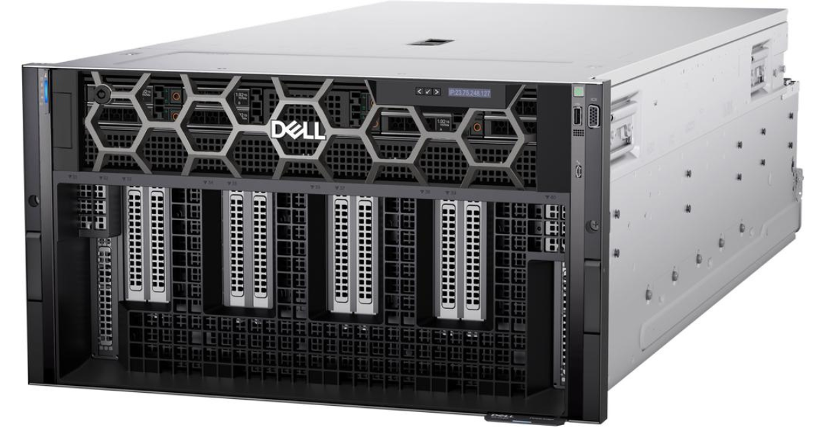
Dell PowerEdge XE9680.
Image source: infohub.delltechnologies.com
GPU and video memory
When selecting an accelerator, evaluate:
- GPU memory capacity and bandwidth.
- Performance in the model's chosen format.
- The connection method between multiple GPUs.
- Power consumption and cooling requirements.
Capacity determines whether the weights, KV cache, and buffers will fit. Memory bandwidth is especially important during autoregressive generation. Multiple GPUs do not automatically form a shared pool: the software environment must split the model, and data must be transferred between the accelerators. Standard PCIe and a high-speed interconnect can produce different latency even when the total memory capacity is the same.
Central processors
CPUs handle tokenisation, APIs, routing, network operations, and part of the RAG pipeline. When processing documents, they also perform decompression, format conversion, and text chunking.
In addition to the number and performance of the cores, the following are important:
- PCIe lanes;
- GPU placement relative to CPU sockets;
- memory bandwidth;
- NUMA topology;
- the number of available storage devices and network adapters.
For dense configurations, consider AMD EPYC servers and Intel Xeon servers. The choice should be based on platform topology, accelerator and software-stack compatibility, rather than the processor name alone.
System memory and NVMe
RAM is used for model loading, containers, the file cache, vector databases, indexes, document preparation, and adapter storage. Offloading part of the model to RAM can make an oversized configuration start, but continuous transfers over PCIe usually increase latency.
NVMe storage mainly affects cold starts, model switching, RAG indexes, and batch processing. If generation, the vector database, and indexing run on the same server, their I/O should preferably be separated across drives or storage pools.
Network
For a text API, the client connection is rarely the main bottleneck. The network becomes more critical when the vector database is on another node, the model is distributed across servers, or several nodes exchange large amounts of data. Latency and stability matter as much as gigabits per second.
Power, chassis, and cooling
Check the following:
- the form factor and power rating of supported GPUs;
- risers, cables, and spacing between cards;
- total power consumption;
- the rack's permitted power capacity;
- whether clock speeds are sustained under prolonged load;
- operation after a power-supply failure.
Specialised platforms are more suitable for several full-size accelerators. The Dell PowerEdge 16th-generation and Dell PowerEdge 17th-generation ranges contain systems of different classes, but compatibility must be checked for the specific chassis, GPU type, and thermal design power.
Why the software environment matters as much as the hardware
Identical GPUs can deliver different performance because of the scheduler and memory-management implementation. Modern inference environments use:
- continuous batching;
- paged KV-cache allocation;
- shared-prefix caching;
- chunked processing of long contexts;
- quantisation;
- model parallelism across GPUs;
- multiple replicas;
- speculative decoding;
- separate queues for interactive and background tasks.
These features are described in the vLLM documentation, but every optimisation has limitations. Shared-prefix caching is useful only when the prefix is repeated. Large batches increase aggregate throughput but may worsen time to first token. Splitting the model adds communication between GPUs, while speculative decoding requires additional memory. Settings should be selected using measurements from the actual workload. (vLLM)
Most popular GPU

Free shipping on orders over £500 in the EU, £500 in the UK, and $3,000 in the USA
Free shipping on orders over £500 in the EU, £500 in the UK, and $3,000 in the USA

Free shipping on orders over £500 in the EU, £500 in the UK, and $3,000 in the USA

Free shipping on orders over £500 in the EU, £500 in the UK, and $3,000 in the USA
Choosing the Right Equipment
Our specialists will contact you and answer all your questions
Calculating the configuration step by step
First, specify the exact model, weight format, and attention architecture. Then:
- Calculate the theoretical weight size and measure actual consumption after loading.
- Determine the median, 95th percentile, and limit for both input and output.
- Calculate the KV cache for the typical peak and for the heaviest permitted request.
- Estimate input- and output-token throughput.
- Choose model parallelism or independent replicas.
- Validate the result with a load test after warm-up.
Calculate input and output throughput separately:
Input tokens/s = requests/s × average input length
Output tokens/s = requests/s × average response length
A long input increases context-processing time and time to first token. A long response keeps the request active for longer and increases concurrent load.
Example calculation for a 70B model
Input data:
- 70 billion parameters;
- 4-bit weights;
- average input — 4,000 tokens;
- 95th percentile — 8,000 tokens;
- average response — 300 tokens;
- one request per second;
- approximately 20 active sequences;
- the 16-bit KV cache from the example above.
The weights theoretically occupy about 35 GB. The KV cache for one sequence of 8,000 tokens is approximately 2.44 GiB, and for twenty sequences it is about 48.8 GiB. The total already exceeds 83 GB before quantisation metadata, buffers, and reserve are included.
A single 80 GB GPU cannot guarantee this workload at the 95th percentile. Several solutions are possible:
- an accelerator with more memory;
- two connected GPUs;
- a lower context limit;
- fewer active sequences per replica;
- a separate pool for long requests;
- several replicas with users distributed between them.
Throughput will be approximately 4,000 input tokens and 300 output tokens per second. These figures define the test profile but do not predict the latency of a particular GPU: that must be measured using the selected model and software environment.
Configurations for different workloads
| Scenario | Main risk | Priority |
|---|---|---|
| Internal chatbot | An unnecessarily expensive server that remains idle | Fast first token, limited history |
| RAG system | Long context and KV-cache growth | Chunk selection, RAM, and NVMe |
| Product API | Queues and unstable latency | Replicas, limits, redundancy |
| Batch processing | The GPU waits for data preparation | Large batches and fast data delivery |
| Multi-tenant platform | Models compete for memory | Separate pools, quotas, and routing |
Internal chatbot
For a small corporate assistant, one GPU with 24–48 GB may be sufficient if the model is compact, conversation history is limited, and few dialogues are active at the same time. If downtime is unacceptable, a second replica is required even when one provides enough performance.
RAG system
The context includes the system prompt, the question, conversation history, and retrieved documents. Limit the number of chunks, and use filtering and reranking. The vector database and generation service do not have to run on the same node, particularly when indexing is resource-intensive.
Product API
Scale replicas with measured useful throughput, not simply “the total number of GPUs.” Set limits on input length, output length, and concurrency for clients. Zero-downtime updates require an additional warmed-up replica.
Batch processing
Higher latency for an individual job is acceptable here, so batching can be more aggressive. The CPU and NVMe storage must feed data fast enough to keep the GPU busy. The background queue should be separated from the interactive queue.
Multi-tenant platform
Several models and adapters compete for GPU memory. Separate pools, token and concurrency quotas, context-length-based routing, and capacity reserved for a node failure are required. It is often more efficient to use several independent replicas than to combine every GPU under one model.
Several GPUs or several servers
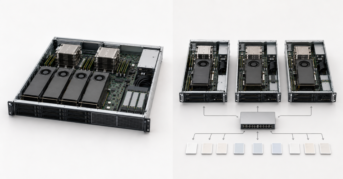
Several GPUs in one server are selected when the model does not fit on one accelerator or when a single large instance needs to be accelerated. Check the connection between the GPUs, support for the chosen type of parallelism, power, and cooling.
Several replicas are preferable when the model fits on one GPU but more users need to be served. This architecture is easier to scale by adding another replica, supports updates without a complete shutdown, and keeps the service running if one accelerator fails.
A single model should be distributed across servers only when one server cannot provide enough resources. This architecture depends on a fast internal network and is more difficult to operate; it is rarely the optimal choice for small and medium-sized models.
Calculation errors
Configurations are most often underestimated because teams:
- count only the weight file;
- use average load instead of peak load;
- multiply the maximum context by all registered users;
- forget the KV cache and response length;
- compare tests with different inputs;
- fill almost all GPU memory with weights;
- assume that a 4-bit model is automatically four times faster;
- mix RAG indexing with the interactive API;
- ignore PCIe topology, power, and cooling;
- test the system with one short request;
- do not provide a standby replica.
An LLM inference server should be selected in the following order: describe the workload profile, calculate the weights and KV cache, determine token throughput, choose the GPU architecture, and only then configure the CPU, RAM, NVMe storage, network, and chassis. The memory calculation answers whether the workload will fit. Only a load test of the specific model in the selected software environment can answer whether the latency and user-capacity targets will be met.
Choosing the Right Equipment
Our specialists will contact you and answer all your questions
Content:
Free shipping on orders over £500 in the EU, £500 in the UK, and $3,000 in the USA
Free shipping on orders over £500 in the EU, £500 in the UK, and $3,000 in the USA
Free shipping on orders over £500 in the EU, £500 in the UK, and $3,000 in the USA
Free shipping on orders over £500 in the EU, £500 in the UK, and $3,000 in the USA

Free shipping on orders over £500 in the EU, £500 in the UK, and $3,000 in the USA
Free shipping on orders over £500 in the EU, £500 in the UK, and $3,000 in the USA